

Common · Literature
Pole–zero plot
In mathematics, signal processing and control theory, a pole–zero plot is a graphical representation of a rational transfer function in the complex plane which helps to convey certain properties of the system such as: Stability Causal system / anticausal system Region of convergence (ROC) Minimum phase / non minimum phase A pole-zero plot shows the location in the complex plane of the poles and zeros of the transfer function of a dynamic system, such as a controller, compensator, sensor, equalizer, filter, or communications channel. By conventi...
From Wikipedia
In mathematics, signal processing and control theory, a pole–zero plot is a graphical representation of a rational transfer function in the complex plane which helps to convey certain properties of the system such as: Stability Causal system / anticausal system Region of convergence (ROC) Minimum phase / non minimum phase A pole-zero plot shows the location in the complex plane of the poles and zeros of the transfer function of a dynamic system, such as a controller, compensator, sensor, equalizer, filter, or communications channel. By convention, the poles of the system are indicated in the plot by an X while the zeros are indicated by a circle or O. A pole-zero plot is plotted in the plane of a complex frequency domain, which can represent either a continuous-time or a discrete-time system: Continuous-time systems use the Laplace transform and are plotted in the s-plane: s = σ + j ω {\displaystyle s=\sigma +j\omega } Real frequency components are along its vertical axis (the imaginary line s = j ω {\displaystyle s{=}j\omega } where σ = 0 {\displaystyle \sigma {=}0} ) Discrete-time systems use the Z-transform and are plotted in the z-plane: z = A e j ϕ {\displaystyle z=Ae^{j\phi }} Real frequency components are along its unit circle
Text: Wikipédia, CC BY-SA 4.0. ·
Related cards
-
 ★
★
Precision approach radar
Type of radar device in aviation
-
 ★★
★★
Differential signalling
Method for electrically transmitting information using two complementary signals
-
 ★★★
★★★
Eigenvalues and eigenvectors
Vectors that map to their scalar multiples, and the associated scalars
-
G★
Generalized Poincaré conjecture
Topological conjecture
-
 ★
★
Percolation threshold
Threshold of percolation theory models
-
 ★
★
Sinusoidal projection
Pseudocylindrical equal-area map projection
-
 ★★
★★
Symmetry (physics)
Feature of a system that is preserved under some transformation
-
 ★★
★★
Poisson point process
Random mathematical object that consists of points randomly located on a mathematical space
-
 ★★
★★
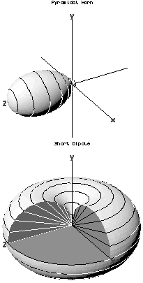
Radiation pattern
Electromagnetism
-
 ★★
★★
Linear function
Mathematical function capturing proportionality
-
 ★
★
Mittag-Leffler's theorem
Theorem about the existence of meromorphic functions with prescribed poles
-
J★★★★
Jacobian conjecture
Conjecture asserting that, over a characteristic-zero field K, given a polynomial map f: Kⁿ → Kⁿ, if its Jacobian determinant J: Kⁿ → K is a nonzero constant map, then f admits a polynomial inverse g: Kⁿ → Kⁿ
-
S★★
Sensitivity analysis
Study of uncertainty in the output of a mathematical model or system
-
W★
Whittaker–Shannon interpolation formula
Signal (re-)construction algorithm
-
 ★★★
★★★
Nyquist–Shannon sampling theorem
Theorem in signal processing describing discrete samples of a continuous signal
-
 ★
★
Pylon turn
Flight maneuver in which an aircraft banks into a circular turn around a fixed spot on the ground
-
 ★
★
Variogram
Spacial statistics function
-
M★
Minimal polynomial (linear algebra)
Minimal polynomial of a matrix