

Direct numerical simulation
Simulation in computational fluid dynamics
A direct numerical simulation (DNS) is a simulation in computational fluid dynamics (CFD) in which the Navier–Stokes equations are numerically solved without any turbulence model. This means that the whole range of spatial and temporal scales of the turbulence must be resolved.
Nº Q1227572 ★
Common · History
Direct numerical simulation
Simulation in computational fluid dynamics
A direct numerical simulation (DNS) is a simulation in computational fluid dynamics (CFD) in which the Navier–Stokes equations are numerically solved without any turbulence model. This means that the whole range of spatial and temporal scales of the turbulence must be resolved.
From Wikipedia
A direct numerical simulation (DNS) is a simulation in computational fluid dynamics (CFD) in which the Navier–Stokes equations are numerically solved without any turbulence model. This means that the whole range of spatial and temporal scales of the turbulence must be resolved. All the spatial scales of the turbulence must be resolved in the computational mesh, from the smallest dissipative scales (Kolmogorov microscales), up to the integral scale L {\displaystyle L} , associated with the motions containing most of the kinetic energy. The Kolmogorov scale, η {\displaystyle \eta } , is given by η = ( ν 3 / ε ) 1 / 4 {\displaystyle \eta =(\nu ^{3}/\varepsilon )^{1/4}} where ν {\displaystyle \nu } is the kinematic viscosity and ε {\displaystyle \varepsilon } is the rate of kinetic energy dissipation. On the other hand, the integral scale depends usually on the spatial scale of the boundary conditions. To satisfy these resolution requirements, the number of points N {\displaystyle N} along a given mesh direction with increments h {\displaystyle h} , must be N h > L , {\displaystyle Nh>L,\,} so that the integral scale is contained within the computational domain, and also h ≤ η , {\displaystyle h\leq \eta ,\,} so that the Kolmogorov scale can be resolved. Since ε ≈ u ′ 3 / L , {\displaystyle \varepsilon \approx {u'}^{3}/L,} where u ′ {\displaystyle u'} is the root mean square (RMS) of the velocity, the previous relations imply that a three-dimensional DNS requires a number of mesh points N 3 {\displaystyle N^{3}} satisfying N 3 ≥ R e 9 / 4 = R e 2.25 {\displaystyle N^{3}\geq \mathrm {Re} ^{9/4}=\mathrm {Re} ^{2.25}} where R e {\displaystyle \mathrm {Re} } is the turbulent Reynolds number: R e = u ′ L ν . {\displaystyle \mathrm {Re} ={\frac {u'L}{\nu }}.} Hence,...
Text: Wikipédia, CC BY-SA 4.0. ·
Related cards
-

Computational fluid dynamics
Branch of fluid mechanics that uses numerical analysis and data structures to solve and analyze problems that involve fluid flows
Nº Q815820 ★★
Not listed
-

Large eddy simulation
Mathematical model for turbulence
Nº Q1755722 ★
Not listed
-
L
Lattice Boltzmann methods
Class of computational fluid dynamics methods
Nº Q1807064 ★
Not listed
-
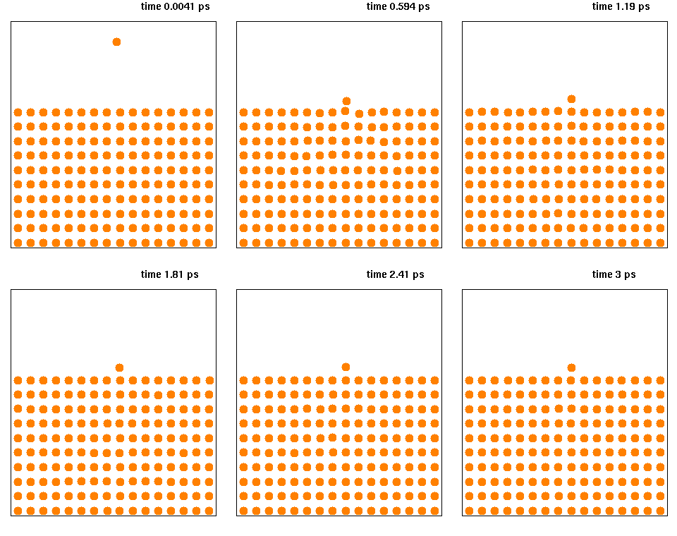
Molecular dynamics
Method of computer simulation of molecular interaction
Nº Q901663 ★★
Not listed
-
L
LS-DYNA
Commercial FEA code
Nº Q570519 ★
Not listed
-
N
Numerical relativity
Sub-area of scientific computing for solving general relativity equations
Nº Q10359034 ★
Not listed